A Level 9618 · Paper 3 · 18.1
Artificial Intelligence: Graphs, Dijkstra and A*
How graphs help an AI find the best route, using Dijkstra's algorithm and A* search. Read the notes, try the past-paper questions, then check the mark scheme.
Past papers from June 2021 to June 202613 questions · 56 marks
Section 18 is one subtopic in the syllabus (18.1). It is split in two here to match the topical booklets: graphs and search, then machine learning.
In this subtopic
- What a graph is, and why AI uses graphs
- Dijkstra's algorithm, traced step by step
- A* search and heuristics
18.1 · 1 of 13Book page Contents
Graphs: nodes, edges and routes
A graph is a collection of nodes (also called vertices) with edges between some of them. Each node has a name. An edge can have a label, which is a number.
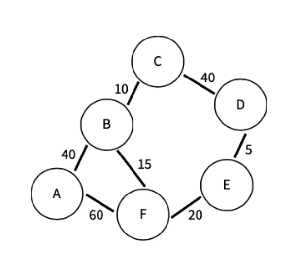
A graph can represent many different situations. A common one is that the nodes are places and the edge labels are the distances between them. An edge is only drawn when you can travel directly between that pair of places. A graph like this can be used, for example, to find the shortest route between two nodes that are not next to each other.
We could use our own intelligence to find the shortest route from node A to node D: list every possible route and add up the distance of each one.
| Route | Overall distance |
|---|---|
| A to B to C to D | 40 + 10 + 40 = 90 |
| A to B to F to E to D | 40 + 15 + 20 + 5 = 80, the shortest |
| A to F to E to D | 60 + 20 + 5 = 85 |
| A to F to B to C to D | 60 + 15 + 10 + 40 = 125 |
For a graph with 100 nodes, this would take far too long. Luckily, a number of artificial intelligence algorithms have been developed to solve this kind of problem.
Practise this: past-paper questions
18.1 · 2 of 13Book page Contents
Why graphs are used in AI
Builds on
Graphs are useful in AI because they give a structure to relationships between things, and many AI problems can be turned into finding a path through a graph.
Graphs in AI
- Artificial neural networks can be represented using graphs.
- Graphs provide structures for relationships, or graphs provide relationships between nodes.
- AI problems can be defined or solved as finding a path in a graph.
- Graphs may be analysed or ingested by a range of algorithms, for example A* or Dijkstra’s algorithm.
- Graphs are used in machine learning.
- An example of a method: back propagation of errors, or regression methods.
Practise this: past-paper questions
Used later in
18.1 · 3 of 13Book pages Contents
Dijkstra’s algorithm
Dijkstra’s algorithm finds shortest paths in a graph. For example, it can be used to work out the shortest distance between two towns.
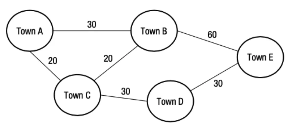
Take the problem of finding the shortest distance from Town A to Town E. On a small graph like this, we could simply use trial and error:
| Possible route | Distance | Total distance |
|---|---|---|
| A to B to E | 30 + 60 | 90 |
| A to C to B to E | 20 + 20 + 60 | 100 |
| A to C to D to E | 20 + 30 + 30 | 80 |
| A to B to C to D to E | 30 + 20 + 30 + 30 | 110 |
The table shows every possible route that does not go round a circuit. The shortest path is A to C to D and then to E, a distance of 80.
As a quick reminder, graphs are made of vertices (or nodes) and edges, which are the connections between them. Some vertices are not connected, so there is no edge between them. A weighted graph, like the one above, has a value (a weight) on each edge.
Dijkstra’s algorithm works out the shortest path from a single source (the starting vertex) to every other vertex. So it also gives the shortest path from the starting vertex to any one destination vertex, as in the example above. It only works on weighted graphs with positive values on the edges.
In one line
- Dijkstra’s algorithm finds the shortest path from one start vertex to every other vertex in a weighted graph.
Practise this: past-paper questions
- June 2023 · Paper 31 · Q2(b)Describe the purpose of both the A* algorithm and Dijkstra’s algorithm
- June 2025 · Paper 33 · Q10(a)State the purpose of the A* and Dijkstra’s algorithms
- November 2025 · Paper 31 · Q7(a)Identify one Artificial Intelligence (AI) algorithm to find the shortest distance between two points on a graph
Used later in
18.1 · 4 of 13Book page Contents
Where shortest paths are used
Builds on
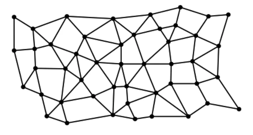
Many common applications need a shortest path algorithm, and Dijkstra’s algorithm is likely to be the basis of all of these:
- Geographic information systems (GIS), such as satellite navigation systems and mapping software. The vertices are geographical locations and the edges show the distance or the drive time.
- Telephone and computer network planning. The vertices are the devices on the network, and the edges could be the physical distance or a measure of what the network can carry, such as bandwidth.
- Network routing and packet switching. The vertices are network devices and the edges are the connections between them. The algorithm can be used to send data packets along the most efficient route. In fact, there is a routing protocol for TCP/IP networks called OSPF, which stands for open shortest path first.
- Logistics and scheduling. Wherever there is a large network of vehicles, such as delivery vans, buses or aeroplanes, the algorithm can be used to calculate the best routes.
18.1 · 5 of 13Book page Contents
How Dijkstra’s algorithm works
Builds on
Here is how the algorithm works on the graph in the next section, where we want the shortest path from vertex A to vertex G (rather than from A to every vertex).
- Start from the first vertex, in this case A.
- Work out the weight (also called the cost) of each edge between that vertex and the vertices it is joined to. For example, A to B is 2 and A to C is 5.
- Move on to the next nearest vertex and repeat. Here it is B. This time you add the weights together to get a total weight from the start. For example, A to B to C is 2 + 4 = 6, and A to B to F is 2 + 7 = 9.
- There are now two ways to get from A to C: direct, with a weight of 5, or A to B to C, with a weight of 6.
- As we want the shortest path, we now know the best route from A to C is direct. Keep this and ignore any longer routes.
- Repeat until every vertex has been visited and you reach the destination vertex, in this case G.
The rule that makes it work
- Each time, the next vertex to visit is the unvisited vertex with the smallest total distance from the start.
- A total distance is only replaced when a new route gives a smaller total.
Practise this: past-paper questions
- June 2021 · Paper 31 · Q5(a)Calculate the shortest distance between the base and each of the other towns in the diagram using Dijkstra’s algorithm. Show your working and…
- November 2023 · Paper 32 · Q8Calculate the shortest distance between the Start and each of the destinations in the diagram using Dijkstra’s algorithm. Show your working and…
- November 2025 · Paper 33 · Q8Calculate the shortest distance between the Start node and each of the nodes in the graph using Dijkstra’s algorithm. Show your working on the…
- June 2026 · Paper 31 · Q9(b)Calculate the best path between the Begin node and each of the nodes in the diagram using Dijkstra’s algorithm. Show your working and write your…
18.1 · 6 of 13Book pages Contents
Tracing Dijkstra’s algorithm
Builds on
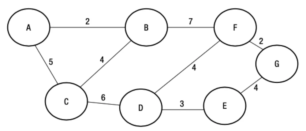
The working gets more complicated because you must keep a running total of the weights along each route, and then choose the shortest. The table traces each stage of the algorithm. Each entry shows the shortest total distance from A found so far, with the vertex it came from in brackets. Bold entries are final: that vertex has been visited and will not change.
| Step | Vertex | A | B | C | D | E | F | G |
|---|---|---|---|---|---|---|---|---|
| 1 | A | 0 (A) | 2 (A) | 5 (A) | ∞ | ∞ | ∞ | ∞ |
| 2 | B | 0 (A) | 2 (A) | 5 (A) | ∞ | ∞ | 9 (B) | ∞ |
| 3 | C | 0 (A) | 2 (A) | 5 (A) | 11 (C) | ∞ | 9 (B) | ∞ |
| 4 | F | 0 (A) | 2 (A) | 5 (A) | 11 (C) | ∞ | 9 (B) | 11 (F) |
| 5 | G | 0 (A) | 2 (A) | 5 (A) | 11 (C) | ∞ | 9 (B) | 11 (F) |
Worked example: Dijkstra’s algorithm
Find the shortest path from A to G, one row of the table at a time.
- Step 1Place A in the first row and fill in the distance from A to each vertex. A to A is 0, A to B is 2 and A to C is 5. Each is marked with (A) to show which vertex it came from, which matters later. Where there is no edge, the value is infinity (∞). A has no other edges, so A is finished.
- Step 2Move to the next nearest vertex to A, which is B, as it has the lowest value in the row above. B keeps the same value, 2 (A), because we already know this is the shortest path from A to B. The next edge is B to C, which is 4. Add the 2 it took to reach B: 2 + 4 = 6. This is more than the 5 we already have for C, so keep 5 (A): going from A to C direct is shorter than A to B to C. The edge B to F gives 2 + 7 = 9, so F becomes 9 (B). As you move down the rows, always keep the lowest value from the row above, because it is the shortest path found so far.
- Step 3Move to the unvisited vertex with the smallest total distance from A, which is C (5). The vertices already visited (A and B) are finished and are not worked out again. The edge C to D has a weight of 6. Add the 5 it took to reach C: 11, so D becomes 11 (C). Apart from D, C has no edges to unvisited vertices, so E and G stay at infinity. C has no edge to F, so F keeps 9 (B): A to B to F is shorter than going through C (A to C to D to F would be 17).
- Step 4Move to the next nearest vertex, which is F (9). It is nearer than D (11), so it goes first. F joins G with a weight of 2. Add the 9 it took to reach F: 11, so G becomes 11 (F). The edge F to D gives 9 + 4 = 13, which is more than 11, so D keeps 11 (C).
- Step 5G (11) is now the nearest unvisited vertex, level with D (11). G is the destination, so the trace stops here and the last row gives the final values. The shortest path from A to G is 11. Follow the letters in brackets back from G: G came from F, F from B and B from A, so the route is A, B, F, G.
Note D and E are not finished in this table, because we only wanted the path to G. A full run of Dijkstra’s algorithm, which finds the shortest path to every vertex, carries on: D stays at 11 (A, C, D) and E becomes 14 (A, C, D, E). E is not really unreachable.
You can check the answer by working out the total weight of every other route from A to G that does not go round a circuit. All of them are longer than 11:
| Other route from A to G | Total weight |
|---|---|
| A, C, D, F, G | 5 + 6 + 4 + 2 = 17 |
| A, B, C, D, F, G | 2 + 4 + 6 + 4 + 2 = 18 |
| A, C, B, F, G | 5 + 4 + 7 + 2 = 18 |
| A, C, D, E, G | 5 + 6 + 3 + 4 = 18 |
| A, B, C, D, E, G | 2 + 4 + 6 + 3 + 4 = 19 |
| A, B, F, D, E, G | 2 + 7 + 4 + 3 + 4 = 20 |
| A, C, B, F, D, E, G | 5 + 4 + 7 + 4 + 3 + 4 = 27 |
Practise this: past-paper questions
- June 2021 · Paper 31 · Q5(a)Calculate the shortest distance between the base and each of the other towns in the diagram using Dijkstra’s algorithm. Show your working and…
- November 2023 · Paper 32 · Q8Calculate the shortest distance between the Start and each of the destinations in the diagram using Dijkstra’s algorithm. Show your working and…
- November 2025 · Paper 33 · Q8Calculate the shortest distance between the Start node and each of the nodes in the graph using Dijkstra’s algorithm. Show your working on the…
- June 2026 · Paper 31 · Q9(b)Calculate the best path between the Begin node and each of the nodes in the diagram using Dijkstra’s algorithm. Show your working and write your…
18.1 · 7 of 13Book page Contents
The A* search algorithm
The A* search algorithm builds on the ideas of Dijkstra’s shortest path algorithm to find the shortest path between two nodes faster. It does this by adding a heuristic, which helps it decide which node to look at next as it moves along the path.
Dijkstra’s algorithm finds the shortest path from the start node to every other node. As well as being faster, the A* algorithm is different because it only looks for the shortest path from the start node to one target node.
| Dijkstra’s algorithm | A* algorithm | |
|---|---|---|
| Finds | The shortest path from the start node to every other node | The shortest path from the start node to one target node |
| Chooses the next node by | The smallest cost from the start | The smallest cost from the start plus a heuristic estimate of the cost to the target |
| Speed | Slower: it also evaluates paths that will never be the shortest | Usually faster: the heuristic steers it towards the target |
Practise this: past-paper questions
- June 2023 · Paper 31 · Q2(b)Describe the purpose of both the A* algorithm and Dijkstra’s algorithm
- June 2025 · Paper 33 · Q10(a)State the purpose of the A* and Dijkstra’s algorithms
- June 2025 · Paper 33 · Q10(b)Outline the difference between the A* and Dijkstra’s algorithms
- November 2025 · Paper 31 · Q7(a)Identify one Artificial Intelligence (AI) algorithm to find the shortest distance between two points on a graph
18.1 · 8 of 13Book page Contents
Heuristics in A*
Heuristics, sometimes called heuristic functions, give “good enough” answers to very complex problems where finding a perfect answer would take too much time. In A*, the heuristic makes the search faster, and as long as it never overestimates the distance left, A* still finds the shortest path.
One drawback of Dijkstra’s algorithm is that it can, and will, evaluate paths that will never give the shortest route. Imagine finding the shortest route on a map from Karachi to Lahore. Anyone who knows Pakistan’s geography would not bother to look at a route through Quetta.
The trade-off between speed and accuracy matters. In some applications, accuracy is less important than computing time. For example, in a SatNav app, a route that is worked out in seconds and is “short enough” is better than waiting 10 minutes for the perfect route.
The A* algorithm uses a heuristic function to help decide which path to follow next. The heuristic function gives an estimate of the lowest cost from a given node to the target node. The algorithm adds the actual cost from the start node, called g(n), to the estimated cost to the target node, called h(n), and uses the result to choose the next node to evaluate. The step-by-step method below shows this in detail.
Practise this: past-paper questions
18.1 · 9 of 13Book page Contents
Choosing a heuristic function
There is no single best heuristic for path finding, because every application is different. For example, if the cost is a distance, it could be estimated by working out the “straight line” distance between the nodes, perhaps using one of these methods:
- Euclidean distance
- Manhattan distance
But remember that the weights on a graph do not always represent distance.
The heuristic must not overestimate
- It is very important that the heuristic function does not overestimate costs.
- As long as the heuristic gives an estimate that is less than or equal to the actual cost, A* will always find an optimal path, and will usually find it much faster than Dijkstra’s algorithm.
18.1 · 10 of 13Book pages Contents
A*: the example graph, g-score and f-score
Builds on
In this example, you use the A* algorithm on a small graph to find the shortest path from A to F. If you have not studied Dijkstra’s shortest path algorithm yet, start there, because much of the terminology is explained in that topic.
The heuristic function used here is a black box. This means you do not see how it works: the detail is abstracted away, so there is one less thing to think about. The function returns the estimated distance from each node to the target node, F:
| Node | Estimated cost to the target node (h) |
|---|---|
| A | 10 |
| B | 15 |
| C | 5 |
| D | 5 |
| E | 10 |
| F | 0 |
On the graph, each heuristic value (in orange) is written next to its node, so all the information you need for the method is in one place.
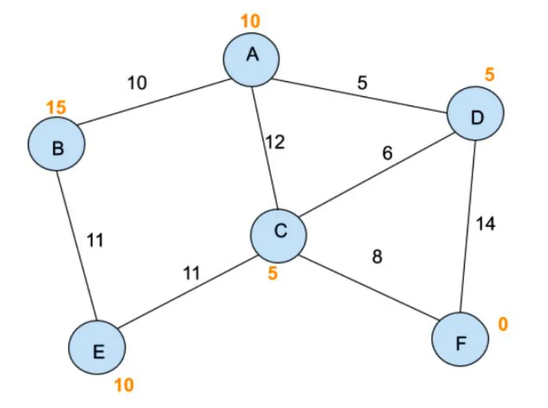
g-score and f-score. In Dijkstra’s algorithm, you kept track of the cost of each path as you evaluated all the possible routes. Every time a shorter path was found, you updated the cost and the previous node.
In A*, the cost of the route from the start node is worked out, stored and updated in the same way, but it is called the g-score. There is also an f-score: the cost of the path so far plus the heuristic’s estimate of the cost to reach the target node. It is the f-score, not the g-score, that is used to choose the next current node.
The three numbers in A*
- g-score, g(n): the actual cost of the path from the start node to node n.
- Heuristic, h(n): the estimated cost from node n to the target node.
- f-score: f(n) = g(n) + h(n). The node with the lowest f-score is chosen next.
Practise this: past-paper questions
- November 2021 · Paper 32 · Q9(b)Find the shortest path between the Home and School nodes using the A* algorithm. Show your working in the table provided. The first two rows in…
- June 2023 · Paper 32 · Q10(b)Calculate the path that takes the shortest time to travel from the Begin node to the End node, using the A* algorithm. Show your working in the…
- June 2026 · Paper 33 · Q9(b)The A* algorithm is used to perform searches on a graph. Calculate the best path between the W and E nodes on the following diagram using the A*…
18.1 · 11 of 13Book pages Contents
Tracing A*: set up, then visit A
Builds on
Step 1: set up the lists. Start by setting the g-score of every node to infinity (or a very large number), to show that it has not been worked out yet. The f-score can also be set to infinity.
- Make the unvisited list with four headings: node, g-score (cost from start), f-score (cost from start + heuristic) and previous.
- In the node column, list every node, starting with the start node (A in this example).
- Set the g-score of the start node, A, to 0 and its f-score to 10, the value the heuristic function returns for A.
- For every other node, set the g-score and f-score to infinity and the previous node to none.
Unvisited list after step 1:
| Node | g-score | f-score | Previous |
|---|---|---|---|
| A | 0 | 10 | none |
| B | ∞ | ∞ | none |
| C | ∞ | ∞ | none |
| D | ∞ | ∞ | none |
| E | ∞ | ∞ | none |
| F | ∞ | ∞ | none |
Now make the visited list with the same four headings. It is empty to begin with and is filled in as the algorithm goes on.
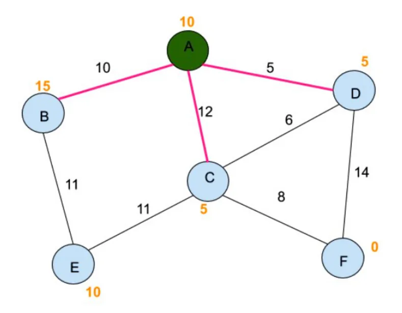
Step 2: A is the current node.
- Pick the node with the lowest f-score in the unvisited list. A has the lowest (10); every other node is infinity. A becomes the current node.
- Look at the nodes that can be reached directly from A (A’s neighbours) that have not been visited yet.
- The edge A to B has a weight of 10. B’s g-score is infinity, and 10 is less, so write 10 and record the previous node as A. h(B) is 15, so B’s f-score is 10 + 15 = 25.
- The edge A to C has a weight of 12. 12 is less than infinity, so write 12 and record the previous node as A. h(C) is 5, so C’s f-score is 12 + 5 = 17.
- The edge A to D has a weight of 5. 5 is less than infinity, so write 5 and record the previous node as A. h(D) is 5, so D’s f-score is 5 + 5 = 10.
- All of A’s neighbours have been looked at. Remove A from the unvisited list and add it to the visited list with its g-score (0), f-score (10) and previous node (none).
Unvisited list after step 2 (the old value is shown after “was”):
| Node | g-score | f-score | Previous |
|---|---|---|---|
| B | 10 (was ∞) | 25 (was ∞) | A |
| C | 12 (was ∞) | 17 (was ∞) | A |
| D | 5 (was ∞) | 10 (was ∞) | A |
| E | ∞ | ∞ | none |
| F | ∞ | ∞ | none |
Visited list after step 2:
| Node | g-score | f-score | Previous |
|---|---|---|---|
| A | 0 | 10 | none |
Practise this: past-paper questions
- November 2021 · Paper 32 · Q9(b)Find the shortest path between the Home and School nodes using the A* algorithm. Show your working in the table provided. The first two rows in…
- June 2023 · Paper 32 · Q10(b)Calculate the path that takes the shortest time to travel from the Begin node to the End node, using the A* algorithm. Show your working in the…
- June 2026 · Paper 33 · Q9(b)The A* algorithm is used to perform searches on a graph. Calculate the best path between the W and E nodes on the following diagram using the A*…
18.1 · 12 of 13Book pages Contents
Tracing A*: visit D, then C
Builds on
This carries on the A* trace from the previous section, on the same graph, from A to F.
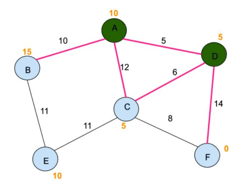
Step 3: D is the current node.
- Pick the node with the lowest f-score in the unvisited list: D (10). D becomes the current node.
- Look at D’s neighbours that have not been visited. You never go back to a node that is already on the visited list.
- The edge D to C has a weight of 6. D’s g-score is 5, so the cost of reaching C through D is 5 + 6 = 11. This is lower than C’s current g-score (12), so update C: g-score 11, previous node D. h(C) is 5, so C’s new f-score is 11 + 5 = 16.
- The edge D to F has a weight of 14. The cost of reaching F through D is 5 + 14 = 19. F’s g-score is infinity, so write 19 and record the previous node as D. h(F) is 0, so F’s f-score is 19 + 0 = 19.
- All of D’s neighbours have been looked at. Remove D from the unvisited list and add it to the visited list with its g-score (5), f-score (10) and previous node (A).
Note By following this method, the unvisited list always holds the lowest g-score and f-score found so far for each node, which is what leads you to the shortest path.
Unvisited list after step 3:
| Node | g-score | f-score | Previous |
|---|---|---|---|
| B | 10 | 25 | A |
| C | 11 (was 12) | 16 (was 17) | D (was A) |
| E | ∞ | ∞ | none |
| F | 19 (was ∞) | 19 (was ∞) | D |
Visited list after step 3:
| Node | g-score | f-score | Previous |
|---|---|---|---|
| A | 0 | 10 | none |
| D | 5 | 10 | A |
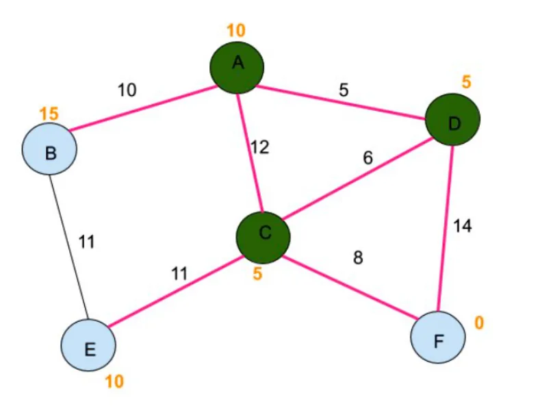
Step 4: C is the current node.
- Pick the node with the lowest f-score in the unvisited list: C (16). C becomes the current node.
- Look at C’s neighbours that have not been visited.
- The edge C to E has a weight of 11. C’s g-score is 11, so the cost of reaching E through C is 11 + 11 = 22. This is less than infinity, so write 22 and record the previous node as C. h(E) is 10, so E’s f-score is 22 + 10 = 32.
- The edge C to F has a weight of 8. The cost of reaching F through C is 11 + 8 = 19. F’s g-score is already 19, and 19 is not less than 19, so nothing changes.
- All of C’s neighbours have been looked at. Remove C from the unvisited list and add it to the visited list with its g-score (11), f-score (16) and previous node (D).
Unvisited list after step 4:
| Node | g-score | f-score | Previous |
|---|---|---|---|
| B | 10 | 25 | A |
| E | 22 | 32 | C |
| F | 19 | 19 | D |
Visited list after step 4:
| Node | g-score | f-score | Previous |
|---|---|---|---|
| A | 0 | 10 | none |
| D | 5 | 10 | A |
| C | 11 | 16 | D |
Practise this: past-paper questions
- November 2021 · Paper 32 · Q9(b)Find the shortest path between the Home and School nodes using the A* algorithm. Show your working in the table provided. The first two rows in…
- June 2023 · Paper 32 · Q10(b)Calculate the path that takes the shortest time to travel from the Begin node to the End node, using the A* algorithm. Show your working in the…
- June 2026 · Paper 33 · Q9(b)The A* algorithm is used to perform searches on a graph. Calculate the best path between the W and E nodes on the following diagram using the A*…
18.1 · 13 of 13Book page Contents
Tracing A*: reach F and read the path
Builds on
Step 5: F is the current node.
- Pick the node with the lowest f-score in the unvisited list: F (19). F becomes the current node.
- F is the target node, so the search is complete. Remove F from the unvisited list and add it to the visited list with its g-score (19), f-score (19) and previous node (D).
- The g-score of F is the cost of the shortest path from A to F: 19.
Final visited list:
| Node | g-score | f-score | Previous |
|---|---|---|---|
| A | 0 | 10 | none |
| D | 5 | 10 | A |
| C | 11 | 16 | D |
| F | 19 | 19 | D |
Finding the shortest path between two nodes.
The visited list holds data for every node that was examined. Notice that, unlike Dijkstra’s algorithm, the A* algorithm does not necessarily give information for every node in the graph, because the heuristic function steers the search towards the target node. In the example, B and E were never visited.
To find the route of the shortest path from A to F, work backwards through the previous nodes:
- Start at F: its previous node is D.
- From D, the previous node is A.
So the shortest path from A to F is A → D → F, with a cost of 19.
Note The route A → D → C → F also costs 5 + 6 + 8 = 19. A* keeps A → D → F because, in step 4, the new cost to F (19) was not less than the one already stored (19). Either route has the shortest cost.
Practise this: past-paper questions
- November 2021 · Paper 32 · Q9(b)Find the shortest path between the Home and School nodes using the A* algorithm. Show your working in the table provided. The first two rows in…
- June 2023 · Paper 32 · Q10(b)Calculate the path that takes the shortest time to travel from the Begin node to the End node, using the A* algorithm. Show your working in the…
- June 2026 · Paper 33 · Q9(b)The A* algorithm is used to perform searches on a graph. Calculate the best path between the W and E nodes on the following diagram using the A*…
18.1
Concepts in 18.1
Every idea explained in 18.1, and where else in the notes it is used.
Zain Merchant's notes, page by page, as printed in his book. The Notes tab has the same notes as text, with links.
Past-paper questions and mark schemes © Cambridge University Press & Assessment. Compiled for revision by Zain Merchant.
- June 2021 · Paper 31 · Q5Notes:Why graphs are used in AIHow Dijkstra’s algorithm worksTracing Dijkstra’s algorithm
- November 2021 · Paper 32 · Q9Notes:A*: the example graph, g-score and f-scoreTracing A*: set up, then visit ATracing A*: visit D, then CTracing A*: reach F and read the path
- June 2023 · Paper 31 · Q2Notes:Dijkstra’s algorithmThe A* search algorithm
- June 2023 · Paper 32 · Q10Notes:A*: the example graph, g-score and f-scoreTracing A*: set up, then visit ATracing A*: visit D, then CTracing A*: reach F and read the path
- November 2023 · Paper 32 · Q8Notes:How Dijkstra’s algorithm worksTracing Dijkstra’s algorithm
- June 2025 · Paper 31 · Q10Notes:Why graphs are used in AI
- June 2025 · Paper 32 · Q6Notes:Graphs: nodes, edges and routes
- June 2025 · Paper 33 · Q10Notes:Dijkstra’s algorithmThe A* search algorithmHeuristics in A*
- November 2025 · Paper 31 · Q7Notes:Dijkstra’s algorithmThe A* search algorithm
- November 2025 · Paper 33 · Q8Notes:How Dijkstra’s algorithm worksTracing Dijkstra’s algorithm
- June 2026 · Paper 31 · Q9Notes:How Dijkstra’s algorithm worksTracing Dijkstra’s algorithm
- June 2026 · Paper 32 · Q9Notes:How Dijkstra’s algorithm worksTracing Dijkstra’s algorithmThe A* search algorithmHeuristics in A*
- June 2026 · Paper 33 · Q9Notes:A*: the example graph, g-score and f-scoreTracing A*: set up, then visit ATracing A*: visit D, then CTracing A*: reach F and read the path
Past-paper questions and mark schemes © Cambridge University Press & Assessment. Compiled for revision by Zain Merchant.
Try the questions first.
Write your answers, then check them against the mark scheme. Your choice is remembered on this device.